Coursera machine learning memo
This holiday break, I somehow got into binge watching Coursera’s Stanford Machine Learning course taught by Andrew Ng. I remember machine learning to be really math heavy, but I found this one more accessible.
Here are some notes for my own use. (I am removing all the fun examples, and making it dry, so if you’re interested in machine learning, you should check out the course or its official notes.)
Intro
Machine learning splits into supervised learning and unsupervised learning.
Supervised learning problems split to regression problem (predict real valued output) and classification problem (predict discrete valued output).
Unsupervised learning problems are the ones we don’t have prior data of right or wrong. An example of unsupervised learning problem is clustering (find grouping among data). Another example is Cocktail Party algorithm (identify indivisual voices given multiple recordings at a party).
Linear regression with one variable
Model representation
x(i) denotes input variables (feature vector), and y(i) denotes the output (target variable). A pair (x(i), y(i)) is called a training example. A list of 1 .. m training example is called a training set.
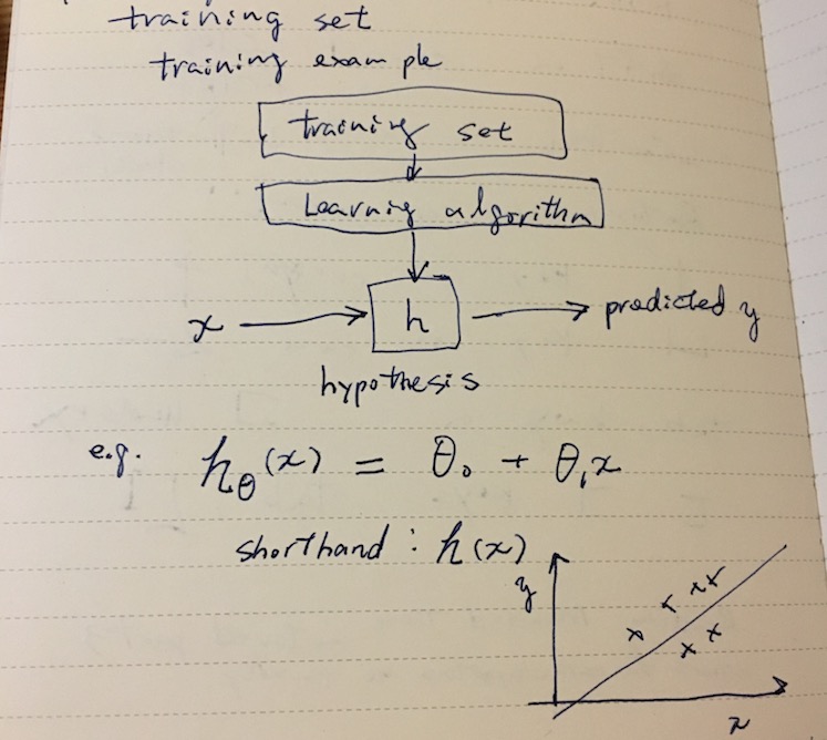
Supervised learning can be modeled as a process of coming up with a good function h called hypothesis that predicts y from an unknown x.
For instance, given square footage, predict price of a house in some city. In the above, hθ(x) is modeled as a linear function. The hypothesis hθ(x) = θ0 + θ1 x is called linear regression with one variable (or univariate linear regression).
These coefficients θ0 and θ1 are called parameters (some textbooks call this w for weight vector).
Cost function
Basically figuring out the parameters θ vector is the name of the game.
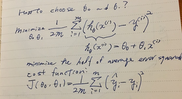
We can turn this into an optimization problem that minimizes the cost function J(θ), which in this case is a mean squared error.
Let’s say a hypothesis is hθ(x) = θ0 x. Depending on the value we put into θ0, it could take different slopes as shown below. To get the intuition for the curve fitting, we can plot the cost function J(θ) against θ.
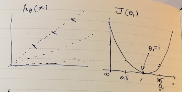
This makes it clear that there’s a single minimum at θ0 = 1.
For two parameter case it might look like a 3D bowl (or more complicated).

For some fixed set of θ0, θ1, hθ(x) is a function of x, and the cost function captures the error between the training examples and the hypothesis.
For two-parameter case, we can try to visualize J(θ0, θ1) using a contour plot, smaller circles showing local maxima/minima.
Gradient descent
Given a hypothesis and its cost function, we can try to find the parameters that fits the data. One of the methods is gradient descent. In gradient descent, the parameters θ0, θ1 are incrementally changed to lower the cost. It turns out that we can determine the direction of walking by taking the partial derivative of J(θ) by θj and multipiled by some learning rate α (η eta is used in textbooks).
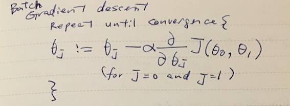
Picking the right α matters here, since if it’s too large you might end up overshooting the target.
Gradient descent for linear regression
Linear regression with one variale is modeled using the hypothesis:
hθ(x) = θ0 + θ1 x
The partial derivative of the cost function looks like this:
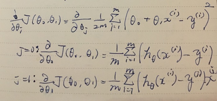
Linear algebra
Skipping the notes on linear algebra section.
- Learn how to multiply matrices and vectors.
Multivariate linear regression
We can expand on the model hθ(x) to incorporate multiple variables. For example, instead of just the size of a house, we can number of bedrooms, age etc.
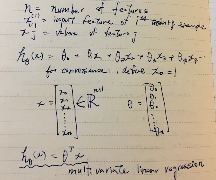
Using vectors θ and x, we can seamlessly build up on dimensions. The trick to express the whole thing as a vector multiplication is to hardcode x0 to 1.
Gradient descent for multivariate linear regression
Here’s how we can find the parameters θ using gradient descent.
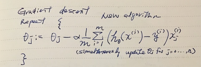
Note that x0 = 1.
Feature scaling
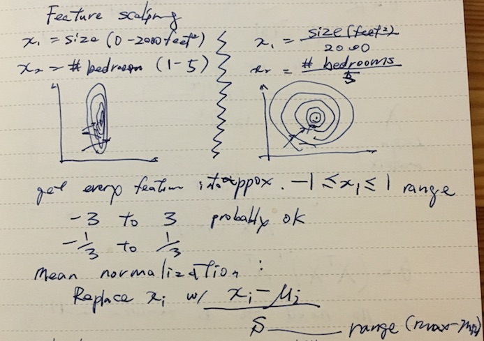
When using gradient descent, it’s important get all the features in the similar scale so the algorithm won’t overshoot. The convention is to get them in the neighborhood of -1 to 1 range, but -3 ~ 3 is considered ok.
Picking the learning rate
If the learning rate α is too small, it’s slow to converge. If it’s too large, it may overshoot and not converge.
To debug this, it’s recommended to plot cost function J(θ) against the number of iterations, and see if it’s dropping fast enough. The suggested increments for α are 0.001, 0.003, 0.01, 0.03, …
Polynomial regression
We can further expand the model hθ(x) for polynomial function. The linear boundaries are straight lines and planes, whereas polynomial can express more complex curves and shaples like ellipsoid.
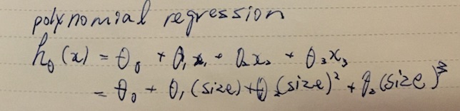
The amazing thing about is that as far as the learning algorithm is concerned, it doesn’t really change anything. We just expand on the feature vector x and add more terms like x02, x03,…
Note that the values are going to be wildly off once you start squaring, so we’d need feature scaling.
Normal equation
Thus far we’ve looked at minimizing J using gradient descent. There’s a second way to calculate this without iteration.
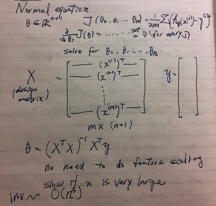
Apparently the slow part is calculating the inverse of a matrix, which is O(n^3).
Vectorization
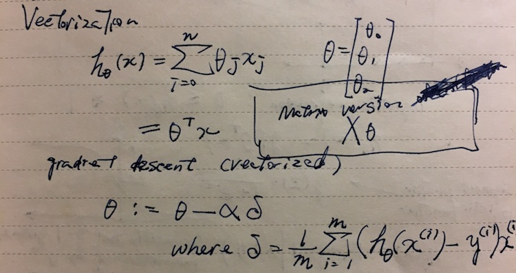
When implementing learning algorithms, avoid using for-loops and try to use vector and matrix multiplications. Generally the process of refactoring to use vector is called vectorization.
When using Octave, I found it useful to use the vectorized application of h(x):
hθ(X) = Xθ
Instead of calculating hθ(x) one row at a time, this calculates the whole matrix in a single shot.
Logistic regression
Classification
Classification predicts discrete class. For instance, filtering email to spam/non-spam.
y ∈ { 0, 1 }
0 is called negative class, and 1 positive class for binary classification problem. There are also multiclass classification problem with more y’s.
One might try to apply linear regression to classfication problem by saying y = 1 when hθ(x) >= 0.5, but apparently it’s not such a good idea.
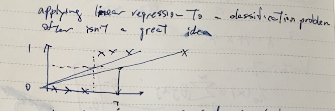
For example, let’s say the x is size of a tumor and y = 1 means malignant, the above shows that adding a large data point can move the decison boundary to the right.
We can setup a better suited model for classification called logistic regression.
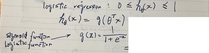
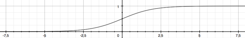
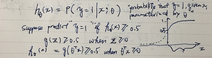
By plugging θTx into logistic function g(z) that gives sigmoid curve, we can turn real values into 0, 1 signal. When z == 0, g(z) returns 0.5. Another way of thinking about this is that hθ(x) will now give us the probability that y = 1.
Decision boundary
Now that we can make hθ(x) to output sigmoid (S-shaped) curve, we can treat hθ(x) >= 0.5 as y = 1. Looking at it from z in g(z), we can say that y = 1 when z >= 0, or θTx >= 0.
So to understand the decision boundary, we can look at where θTx == 0. Here are some examples of the decision boundaries.
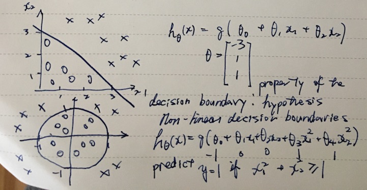
Note that once θ is picked, the decision boundary is a property of the hypothesis function (hθ(x)).
Cost function of logistic regression
The cost function for the logistic regression is a bit involved. We can’t use the same cost function J(θ) apparently because it will cause the output to be wavy (many local optima). Here’s a convex alternative:
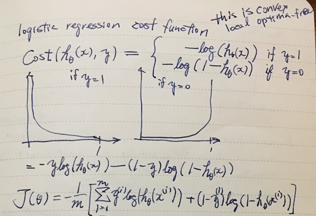
It looks gnarly at first, but remember that y ∈ { 0, 1 }. By multiplying y or (1 - y), half of the term goes away, emulating the “if y = 1” clauses. Another thing to keep in mind is that if hθ(x) somehow manages to compute h(x) = 0 when y = 1, then this cost function will return a whopping penalty of +∞.
The gradient descent is actually surprisingly simple:
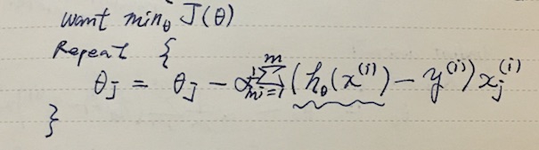
Whatever you plug into hθ(x) is different, but the shape of the algorithm looks identical to that of linear regression version.
Optimization problem
The general problem of minimizing J(θ) for θ is called the optimization problem. Gradient descent is one approach is there are faster ones like conjugate gradient, BFGS, and L-BFGS. In Octave, fminunc is one of the optimizers.
Multiclass classification
To expand the model to deal with y ∈ { 0, 1, …, n }, we take an approach calle one-vs-all where we divide the problem into n + 1 binary classification problems, and thus n + 1 hypotheses.
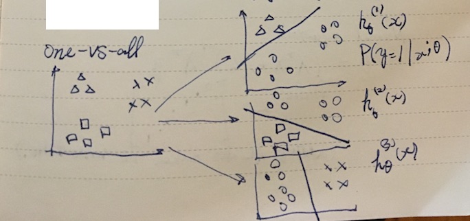
To make a prediction on a new x, pick the class that maximizes hθ(x).